Thomas Rimer
Characterizing Laser Speckle
I explored the effects of optics’ surface roughness on the formation of laser speckle for my Introduction to Experimental Physics Laboratory class.
I prepared all samples, captured all data, processed the photos, and made the final poster. My partners helped with initial ideation on the experiment, and contributed to the final writeup.
Final Poster
Project Details
In this project, I collected images of laser speckle caused by optics with 12 different well-defined surface roughnesses. Using OpenCV, I characterized the intensity distribution of the speckle to confirm that it follows an exponential decrease in intensity for all surface roughnesses.
Introduction
Laser speckle occurs when temporally coherent light shines through a transparent medium with a rough front and/or back surface, leading to the beam constructively and destructively interfering with itself which results in small bright spots in the beam. While speckle is typically avoided in experiments, characterization of speckle is useful not only for understanding how best to mitigate speckle, but can also be used to understand the roughness of the surface itself. While prior literature suggests that speckle intensities follow a negative exponential distribution, investigations into the robustness of the negative exponential distribution across a wide array of surface roughnesses are lacking. The goal of this research project was to investigate how well the negative exponential models speckle intensities across surface roughnesses.
Samples
I sanded 11 1.5” x 1.5” x 0.25” acrylic squares, each with one of the following sandpaper grits: 150, 180, 240, 320, 400, 600, 800, 1000, 1500, 2500, or 3000. All samples were wet sanded in a circular pattern for 3 minutes. Only a single side was sanded. I positioned samples in the mount such that the laser beam entered the sample through the smooth (unsanded side) and exited via the rough (sanded side).
For a given grit sample, 10 photographs were taken, each with the laser shining through a different region of the acrylic square. For each grit, a photograph was also taken while the laser was off, providing a background noise reference which was subtracted from the 10 sample photographs during the processing. An additional 10 samples plus a single background reference were also taken for the control (no sanding) sample. This yielded a total of 132 photographs [11 grits x (10 samples per grit + 1 background) + 1 control grit x (10 samples + 1 background)], resulting in 11.8 GB of raw photographic data (~3.2 billion pixels).
Analysis
All images were processed by an OpenCV program I wrote in Python. The analysis program can be thought of in levels: in total, there were 4 levels: Level 0, Level 1, Level 2, and Level 3. Each level represents a layer of processing away from the original photographs and are explained in detail below. All code and histograms are available on my Github.
Level 0: Raw Images
Prior to ingestion into the Python program, I converted the CR2 raw photos captured by the camera were into a non-proprietary file format easily manipulated with OpenCV. The final PNGs used in the program were approximately 90 MB each. Below are two representative photographs of the original, raw CR2s (the processed PNGs are visibly identical).
Level 1: Individual Histograms
My OpenCV program (written in Python) ingested each photo and created an intensity distribution of pixels in the photograph. First, the ingested photo was converted to greyscale (with the OpenCV cvtColor COLOR_BGR2GRAY function). Weights for the red, green, and blue channels can be found on OpenCV’s website. Next, the intensity of the grayscale image was rescaled such that bit intensities ranged between 0 (dark) and 1 (bright/saturated). The average pixel intensity of the background reference photo for a given grit was also calculated, and subtracted from all values in the original speckle image. To reduce high frequency noise, a Gaussian blur using a 25x25 kernel was applied across the image.
To extract intensities, an equally-weighted 3x3 kernel was convoluted across the image resulting in a 1D array of intensities. Note that this step stripped all spatial information from the photo; no spatial information was used at any subsequent point. The convolved intensities were plotted as a histogram with 100 buckets consistent across all histograms. The bounds of the bucket were linearly spaced. Because camera settings were identical across all photos, the bucket intensities were also identical and thus enabling objective, relative comparison. Below are the histograms for the two representative speckle patterns explained in Level 0.
Level 2: Grit Averaged Exponentials
For each given grit (of which there were 10 samples) the average count and standard deviation was calculated for each bucket. These were plotted as “average” histograms, with the height of each bucket representing the average and the error bars representing the standard deviation.
Next, a curve was fitted to the data. The natural logarithm of each bucket mean was taken and a linear curve of the form mI + b, where m, b are floats and I is the bucket center (intensity) was fitted. The curve was re-exponentiated for plotting. Below are the grit averaged histograms for the same two representative speckles analyzed in the previous two sections.
Level 3: Fit Trend
The slopes from each fit in Level 2 were plotted on a graph against their grit size. Uncertainty for each data point was calculated using covariance matrices from the fits, discussed below. Below is the single, final slope trend graph representing all grits.
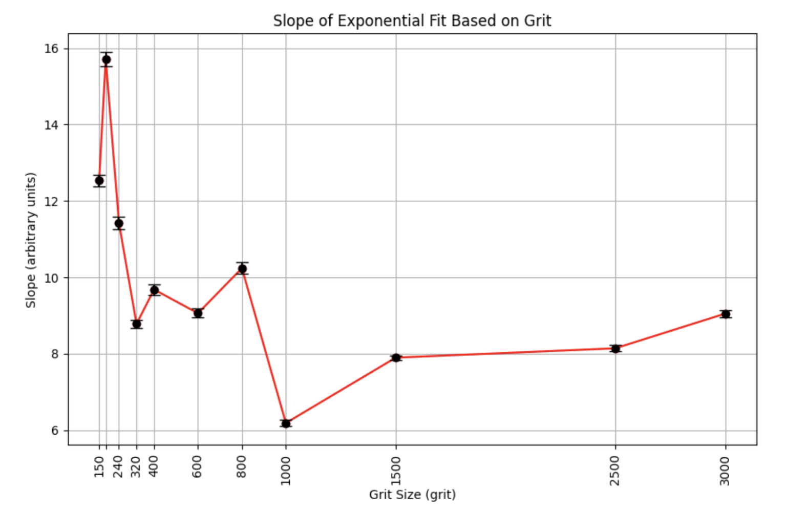
Conclusion
The experiment confirmed that laser speckle intensity distributions, regardless of surface roughness, consistently follow negative exponential trends. A notable outcome was the observed inverse relationship between grit number and fit slope; as surface roughness decreases (i.e. grit increases), speckle patterns narrow and intensify while adhering to an exponential distribution.